Sample Use of web-HUMAN 6
For Lecture Demonstration Purposes

Note: The document below introduces experiment save/retrieve in workshop (screen by screen) format. It was written for Human 6 which differs from Human 6.1 only in the lack of within-the-model on-line help. A refresher page summarizing the differences between 6.0 & 6.1 screen formats is available here.

Below is a sample use of the Save/Retrieve Experiment capabilities of HUMAN 6 drawn from RSM's first attempt to use the model's new capabilities for lecture demonstration purposes. The pedagogical setting was an approximately 50 student lecture hall situation.

0) You are already logged in
This example assumes you are already logged in as a registered user, a condition required for all save/retrieve maneuvers.
If not, click on Login for personalized features at the opening screen & follow the simple instructions to register/login.

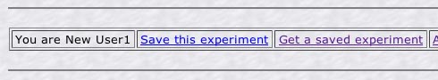
1) You retrieve the lecture demo
Pick the choice Get a saved experiment from the bottom of your screen. (see below)

2) On the Retrieve a Saved Experiment screen (see below) locate the folder Heat Balance Demo and then click on Open folder .

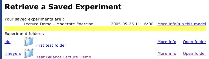
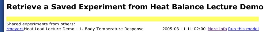
3) You will now see a screen (Retrieve a Saved Experiment From Heat Balance Lecture Demo - below) of the 5 lecture demo files.
Look for 1.Body Temperature Response and click on the More info link.

4) You will see the Information about this experiment screen . Read through it.

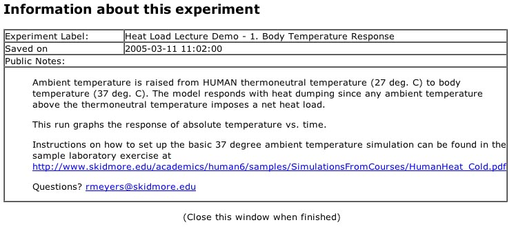
Notice that the basic maneuver is to raise ambient temperature (TEMAB) from 27 degrees C to 37 degrees C (i.e. equal to body temperature, TEMP). This imposes a net heat load on the body and sets up a lecture situation in which the thermoregulatory response to heat loads can be discussed.

5) We now close this window as instructed at the bottom (Close this window when finished) and are back at our main screen.
We choose to Run this model . A graph and a tabular output appear.

6) Examining the tabular output first (click on the tabular screen to bring it to the foreground) we see the screen below.

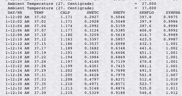
Grasping the gestalt of the response in the table we see that 6 variables were read out in the tables (TEMP, CALP, etc.) as defined below.

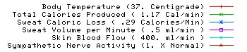
and that they were chosen to illustrate

• a] heat dumping mechanisms - Sweat calories lost, sweat volume, skin blood flow
• b] control of heat dumping - sympathetic nervous system activity and
• c] drivers and costs of the response - body temperature, caloric cost of the response

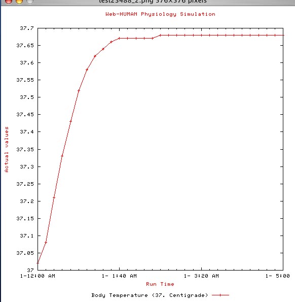
7) That the heat load causes a small rise in the model's temperature until it stabilizes can be seen by clicking on the body temperature graph (see below). This increase in turn drives the increases in evaporative and conductive heat loss.

8) Close the graph and click on the Back button on the Skidmore Web-Human screen to return to the other demo choices (as seen below).

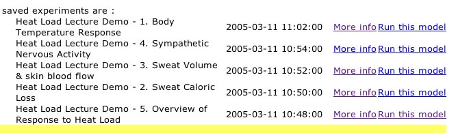
8) Explore these as you wish. They stress various aspects of the response as their titles indicate.